Function Approximation with Taylor Series, Polynomial Regression, and Neural Networks
Project Highlights: Visualization of Taylor Series Approximations, using Linear Regression with Taylor Polynomials to approximate derivatives, visualizing a Neural Network - coded from scratch with Numpy - approximate functions
Function approximation is a fundamental concept in numerical analysis and machine learning, where the goal is to approximate a target function using a simpler or more easily computable form. This project explores three different methods for function approximation: Taylor Series, Linear Regression with Polynomial Terms, and a Neural Network implemented from scratch using Numpy.
Table of Contents
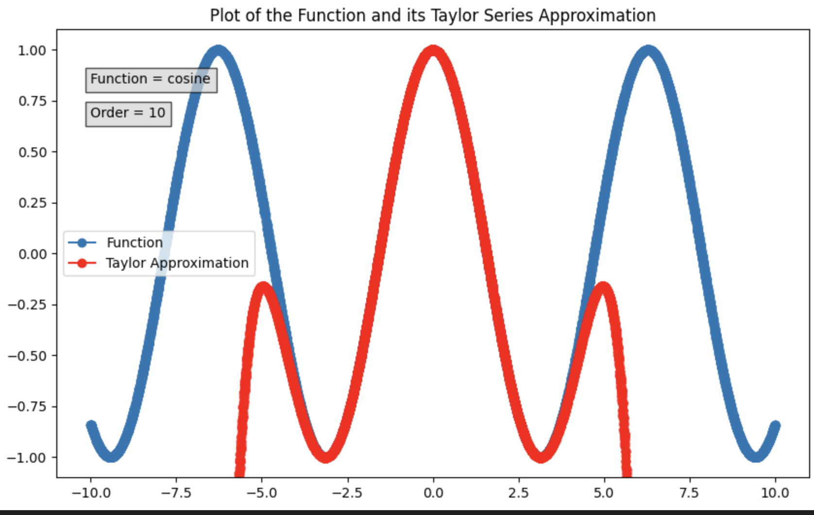
The Taylor series is a representation of a function as an infinite sum of terms calculated from the values of its derivatives at a single point. This method is particularly effective for approximating smooth functions that are well-behaved near the point of expansion.
The Taylor series of a function \( f(x) \) about a point \( a \) is given by: \[ f(x) = f(a) + f'(a)(x-a) + \frac{f''(a)}{2!}(x-a)^2 + \frac{f'''(a)}{3!}(x-a)^3 + \cdots \] Here, \( f'(a) \) is the first derivative of \( f \) at \( a \), \( f''(a) \) is the second derivative, and so on. The series provides an approximation of \( f(x) \) around the point \( a \).
Approximating Cosine
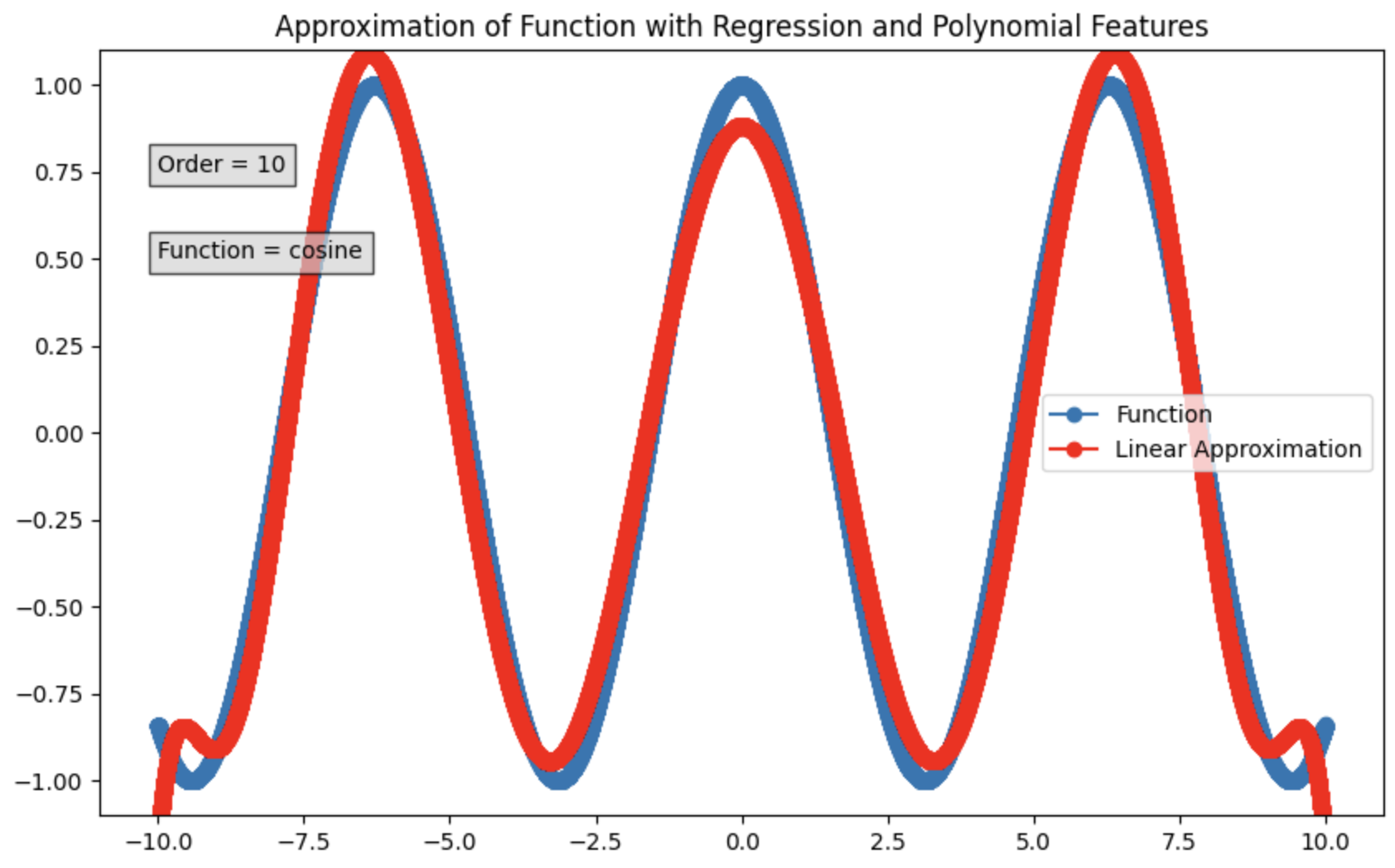
Taylor Series are effective only when you have the function you're approximating and can take its derivatives. But what if that's not the case? We can still leverage the concept of Taylor Polynomials for function approximation. By using polynomial terms as features in a linear regression model, we can estimate the coefficients, which correspond to the function's derivatives. This approach not only approximates the function but also provides an estimation of its derivatives.
Approximating Cosine
| Polynomial Order | Estimated Coefficient |
|---|---|
| 1 | 0.0000 |
| 2 | -1.0000 |
| 3 | 0.0000 |
| 4 | 1.0000 |
| 5 | 0.0000 |
| 6 | 0.9999 |
| 7 | 0.0000 |
| 8 | 0.9994 |
| 9 | 0.0000 |
| 10 | -0.9972 |
| Polynomial Order | Estimated Coefficient |
|---|---|
| 11 | 0.0000 |
| 12 | 0.9885 |
| 13 | 0.0000 |
| 14 | -0.9579 |
| 15 | 0.0000 |
| 16 | 0.8670 |
| 17 | 0.0000 |
| 18 | -0.6536 |
| 19 | 0.0000 |
| 20 | 0.3027 |
Notice how the polynomial terms, centered around 0, closely match the actual derivatives of the cosine function at \( x = 0 \). When we adjust the polynomial to be centered at \( x = 1 \), the first five Taylor polynomial coefficients reflect the following values:
It's important to observe that these coefficients maintain the 4-cycle derivative pattern characteristic of the cosine function.
| Polynomial Order | Estimated Coefficient |
|---|---|
| 1 | -0.8415 |
| 2 | -0.5403 |
| 3 | 0.8415 |
| 4 | 0.5403 |
| 5 | -0.8414 |
Approximating an Unknown Function
Here, I created my own function to approximate. The function is \( f(x) = \sqrt{e^{\frac{x}{10}}} \cdot \cos(x) + 4 \)
The first 3 estimated coefficients for this function are 0.0277, -0.221, and -0.0842. While perhaps a bit tedious, finding the derivative of this function should be something all my former students should have no problem with! The rest of the problem is left to the reader.
Instead of using Taylor polynomials and linear regression for function approximation, I opted for a Fully Connected Neural Network. By coding this neural network from scratch using Numpy, I aimed to deepen my understanding of both the mathematical principles and the vectorization capabilities of Numpy.
My implementation is highly flexible, allowing users to define both the number of layers and the size of each layer. For hidden layers, I employed the ReLU activation function to introduce non-linearity, while the final layer utilizes a linear activation function. All layers are initialized with HE initialization to ensure optimal weight scaling.
I trained the network using whole-batch gradient descent. Initially, I encountered some training challenges, which I resolved by incorporating momentum and learning rate decay. These enhancements significantly improved the network's performance, making it unnecessary to explore more advanced optimizers like RMSProp or Adam, or additional regularization techniques such as weight decay and dropout. The resulting neural network is robust and efficient, delivering precise function approximations.
After some further investigation, the difference in performance between the two purely comes down to the extra layer. When given the same number of layers, the models shared remarkably similar results and rates of learning. Turns out this is not very hard for a Neural Network to approximate.
Notice also that the neural network is able to get extremely precise results with few polynomial terms. Compare the NN's approximation with 10 terms with Taylor Series.
Visualizing Local Critical Points
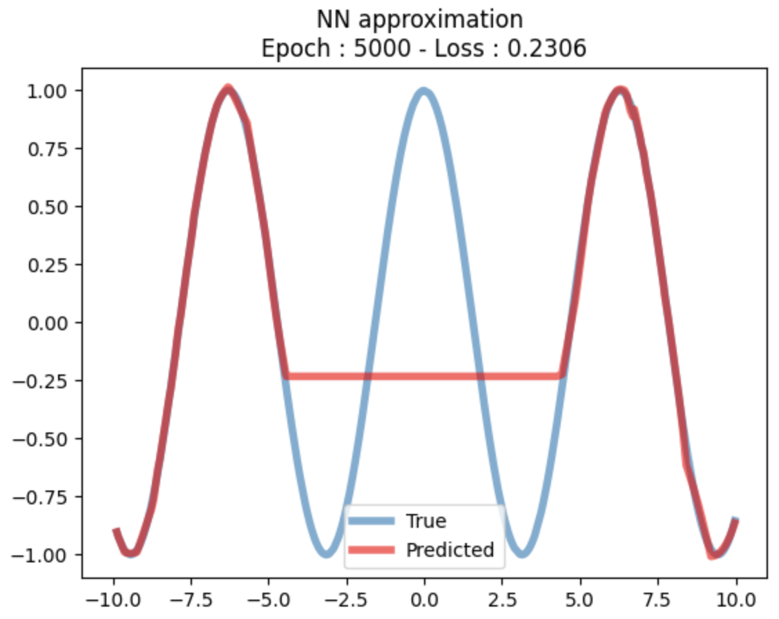
With some instances, I saw the result above. This was a very interesting depiction of a common challenge in training neural networks: getting stuck in local optima. In this scenario, the neural network's predictions do not accurately capture the true underlying function, and instead, the model converges to a suboptimal approximation. This phenomenon occurs when the optimization process stalls in a local minimum of the loss function, preventing the network from finding a more accurate global solution.
With a simple optimizer like gradien descent with momentum, it is easy to get stuck in local optima depending on the initlaization. Initialization plays a crucial role in the training of neural networks and can significantly impact the final model performance. The weights of the network are typically initialized with small random values. The choice of these initial values can influence the trajectory of the optimization process. If the weights are initialized poorly, the network might converge to a local optimum instead of the global optimum, resulting in suboptimal performance.