Understanding and Visualizing the Perceptron Algorithm

First, if you are interested in viewing my Notebook to play around with, click here.

As part of my Machine Learning course with Professor Gabor Lugosi, part of our homework was to code the Perceptron Algorithm from scratch and apply it to generated linearly separable and linearly non separable data across different sample sizes, dimensions, and degrees of separability. This was then compared to the Bayes Risk.

Coding this was quite a fun challenge and gave me admittedly a fondness for this simple algorithm. For sure, the Perceptron is incredibly limited and I didn't understand at first why we were learning such an ancient algorithm. However, it ended up being a great introduction into empirical risk minimization and helped me thinking about data as projections in space in a new light.

Additionally, I added a visualization feature in my algorithm to help me see what the algorithm was doing in two dimensional cases.

Generating the Data

To generate the data for this binary classification problem, I created data from two distributions.

In the linearly separable case, we pull from uniform distributions and we set the degree of separation with alpha.

For the linearly inseparable case, we draw from multivariate normals. However, for the first dimension, we set the mean to be 0 for one class and m for the other class. The means for the rest of the dimensions are 0.

The Algorithm

This algorithm was invented in the 50’s and learns a neuron (a linear classifier is basically a neural network with one neuron).

Suppose that the data is nearly separable. Let’s see the algorithm.

1. We start with an arbitrary \( w_0 \), for example \( w_0 = \vec{0} \).
2. Then we go through our data points one by one.
   At time \( t \):
   • If \( w_{t-1} X_t Y_t > 0 \) then we do nothing.
   • If \( w_{t-1} X_t Y_t \leq 0 \) then \( w_t = w_{t-1} + X_t Y_t \).
3. Stop when all data points are correctly classified. Cycle through the data several times if needed.
   

Linearly separable data is a huge assumption. As we see in the visualization, we must create a maximum number of iterations or else it will run forever (as there will always be at least one misclassified point by definition.)

Results

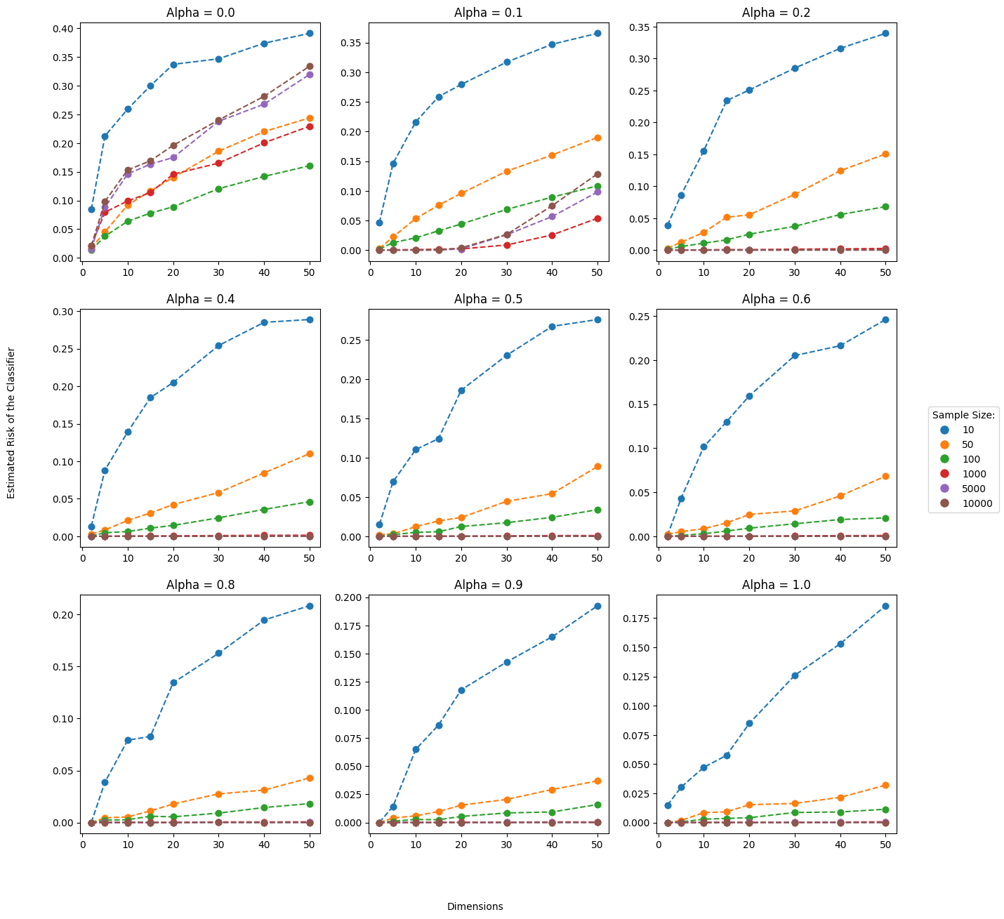
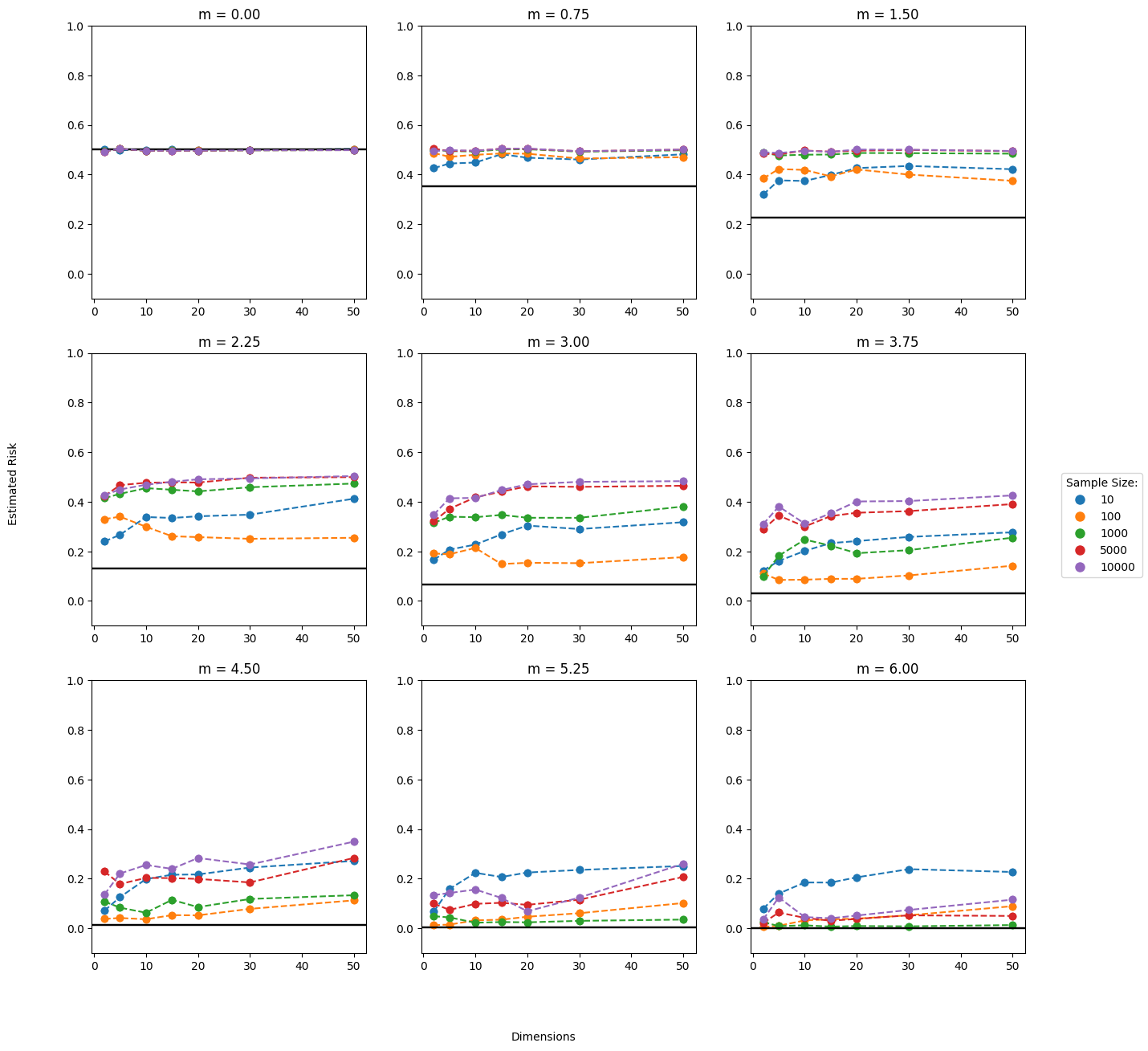
To obtain our results, we tested the perceptron on numerous generated datasets. We tested across different dimensions, sample sizes, and degrees of separability (alpha for separable data and m for nonseparable data as defined above). We tested each combination of parameters 20 times. By using 10,000 generated out of sample testing points, we calculate the average risk (1 - accuracy) to estimate the true risk. See the results below:

Bayes Risk

The Bayes Classifier is the ideal classifier if the distribution of the data is known. The Bayes Risk is simply the expected risk of the Bayes Classifier. For linearly separable data, the Bayes Risk is 0. There is no overlap in the distributions so we know every time which class the data belongs to given the class distributions.

For our case of linearly inseparable data, below my calculations for the Bayes Risk.

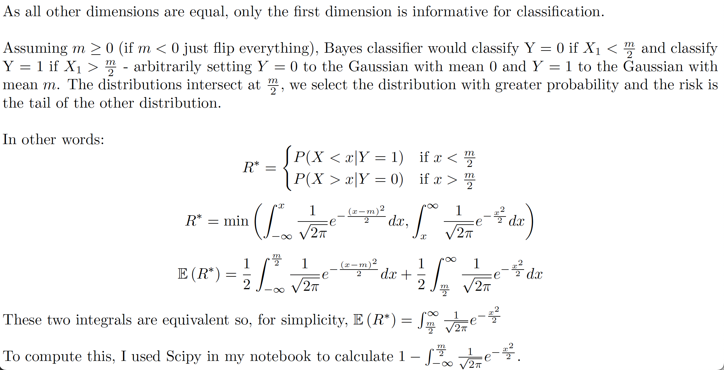
Using this, we can compare our results above to the Bayes Risk as demonstrated by the black line.

Extensions

If you read through all that... Thank you. Here were a couple thoughts of how you can expand on what I did.

Non-Linearly but Separable Data Kernels

What if we kernelized the perceptron classifier? This would be helpful for data that is separable but not necessarily linearly separable. Even for non-separable data, the Bayes classifier here is linear because the covariance matrices for both classes are the same. But what if they weren't?

Support Vector Machines

All the perceptron cares about is separating the data. SVM works differently by trying to maximize the margin. Try doing the same thing with hard-margin SVM and then try it again with soft-margin SVM. Let me know if you do?

Visualization Expansions

Visualize perceptron in 3 dimensions. Then do it in 4 dimensions (just kidding). Also, an improvement on my visualization would be, for each update, the misclassified point in question is highlighted.

If you do any of these, please let me know. I'd love to see! Thanks for reading!